← Back to the post: Consumers Can Handle a Stock Crash
The AI Boom and Its Risks · Part 3 · Online appendix
Online Appendix: Consumers Can Handle a Stock Crash
This appendix accompanies “Consumers Can Handle a Stock Crash,” the third post in The AI Boom and Its Risks. It reviews what economists have found about how much consumer spending responds to changes in household wealth, then documents the estimates behind the post in far more detail than the post itself could. It was written by Claude, an AI model made by Anthropic, at Jason Furman’s direction. He has not edited all of it, so any errors are Claude’s. Code and data to reproduce every number in the post and in this appendix are in the replication package.
The findings in brief
- The literature’s central estimate is about 3 cents of extra annual spending per extra dollar of stock wealth, with most credible estimates between 2 and 4 cents. Housing wealth usually has a somewhat larger effect. Responses to losses and gains are hard to tell apart, and the literature has not found a robust difference. Whether the effect has shrunk over time is contested, and almost nothing published covers the years since 2019.
- A consumption function estimated on 1955–2019 data gives 2.2 cents per dollar of stock wealth and 4.4 cents per dollar of housing wealth. Spending adjusts quickly: about 70 percent of the long-run effect arrives within a year.
- Since 2019 spending has risen less than that function predicts. Starting from 2019, spending in the third quarter of 2026 was 2.1 percent of disposable income ($510 billion a year) below the projection; starting from the 2015–2019 average, 3.6 percent ($870 billion). Only about a quarter of the stock effect the function expected is visible from a 2019 start, and none from a 2015–2019 start, which is the basis for the post’s statement that adjusting for the prediction errors takes the estimate “down to 1 cent or lower.” Measured from 2024, however, spending has kept pace with the function (and nearly so from 2023), so the shortfall is a level that opened up before then, not a gap that keeps widening.
- The miss is within this method’s historical error by itself, but past misses track how much the model expected stocks to add (correlation 0.7), and this time the model expected more from stocks than ever before.
- No asymmetry survives scrutiny. Losses appear to matter more than gains only when the unspent gains since 2019 are lumped in with earlier gains.
- There is no statistically robust evidence that the stock coefficient fell before 2020. Estimates fall sharply only once the years since 2019 are added: from 2.2 cents through 2019 to 1.1 cents through the third quarter of 2026 on all data since 1955, and to 0.6 cents over the latest 20 years.
1. What the literature finds
The marginal propensity to consume out of wealth is the increase in annual consumer spending that follows a one-dollar increase in household wealth, once spending has had time to adjust. It is usually quoted in cents per dollar. Simple life-cycle logic says it should be a few cents: a household that spread an extra dollar evenly over the rest of a 40-year horizon, earning a 3 percent real return, would spend about 4.3 cents a year more. Bequest motives, the age of the people who hold the wealth and doubts about whether a gain will last all push the number lower. When Jason Furman first worked on macroeconomic policy in the mid-1990s, the rule of thumb in policy circles was 1 to 5 cents. Table A1 summarizes the estimates discussed below.
Table A1. Selected Estimates of How Much Spending Rises per Dollar of Wealth
| Study | Data | Stock wealth | Housing wealth | Total wealth |
|---|---|---|---|---|
| Poterba (2000) | Survey of the U.S. evidence | About 3 in the long run (range 1–5); 1–2 in the first year | — | About 3 |
| Ludvigson and Steindel (1999) | U.S. quarterly, 1953–1997 | 4.0 (2.1–10.6 across subperiods) | — | 4.6 |
| Davis and Palumbo (2001) | U.S. quarterly, 1960–2000 | 3.8–5.7 | — | 3–6 |
| Carroll, Otsuka and Slacalek (2011) | U.S. quarterly, 1960–2007 | Financial: 0.8 in the first quarter, 4.1 eventually | 1.8 first quarter, 8.7 eventually | 0.9 first quarter, 4.8 eventually |
| Fair (2017, 2024) | U.S. quarterly, 1954–2023 | About 4 (financial wealth) | About 5 | About 4 |
| Duca, Muellbauer and Murphy (2017) | U.S. quarterly, 1972–2017, with credit conditions | 1.4 (illiquid financial) | About 1 (1980s) to 3.75 (mid-2000s); below 2 (2015) | — |
| Aladangady and Feiveson (2018) | U.S. quarterly, 1960–2007 | — | — | 3.5 |
| Beach, Gamber and Moran (2025) | U.S. quarterly, 1964–2011, tested through 2019 | Slightly above 1 | Just over 5 | 3.5; with a break, 3.3 before 2012 and 2.7 after |
| Slacalek (2009) | 16 countries, quarterly; U.S. 1965–2003 | 5.3 (financial) | 7.0 (imprecise) | 5.4–6.0 |
| Calomiris, Longhofer and Miles (2013) | U.S. states, annual, 1985–2009 | 0–1.8 | 5.5–8.1 | — |
| Chodorow-Reich, Nenov and Simsek (2021) | U.S. counties, quarterly; dividend data 1989–2015 | 3.2 | — | — |
| Andersen, Johannesen and Sheridan (2024) | Danish investors, 2009–2016 | About 4 in the first year (4.4 published) | — | — |
| Di Maggio, Kermani and Majlesi (2020) | Swedish households, 1999–2007 | 2.8 (top 5 percent) to 23 (bottom half) | — | — |
| Mian, Rao and Sufi (2013) | U.S. counties, 2006–2009 | — | 5.4–7.2 | — |
| Guren, McKay, Nakamura and Steinsson (2021) | U.S. metropolitan areas, 1978–2017 | — | 2.4 (3.3 for 1990–2017) in the working paper; about 2.7 in the published article | — |
| This appendix: consumption function | U.S. quarterly, 1955–2019 | 2.2 | 4.4 | 2.5 |
Note: Cents of annual consumer spending per dollar of wealth, long run unless stated. Studies define wealth, spending and income differently, so the numbers are not strictly comparable. Fair’s 2024 re-estimate dummies out 2020–2021.
Sources: The studies listed; author’s calculations for the last row.
1.1 How much people spend out of wealth
The classic estimates come from national time series. Poterba (2000) surveyed them and put the consensus long-run effect at about 3 cents per dollar of stock wealth, within a range of 1 to 5, with 1 to 2 cents showing up in the first year. Ludvigson and Steindel (1999) found about 4 cents for stocks over 1953–1997; Davis and Palumbo (2001), 3 to 6 cents for total wealth over 1960–2000. Ray Fair (2017), who has estimated the same equations for decades, finds about 4 cents per dollar of financial wealth and about 5 per dollar of housing wealth, and his 2024 re-estimation through 2023 (with the pandemic quarters dummied out) leaves the effect at about 4 cents. Carroll, Otsuka and Slacalek (2011) emphasize how sluggish the response is: in their estimates only 0.8 cents per dollar of financial wealth shows up in the first quarter, against 4.1 cents eventually.
Aggregate time series have a well-known weakness. Stock prices move on news about future incomes and profits, so a correlation between stock wealth and spending may reflect households reacting to the same news rather than to their wealth. The most convincing recent estimate gets around this. Chodorow-Reich, Nenov and Simsek (2021) compare U.S. counties whose residents hold a lot of stock relative to their labor income with counties whose residents hold little. Because every county faces the same national market return, the comparison strips out whatever the market is signaling about the national economy. After the market rises, payrolls in retail, restaurants and hotels rise more in the high-wealth counties, implying that households spend 3.2 cents a year per dollar of stock wealth, with about half the response within two quarters and the whole of it within about seven.
Household data show how unevenly that average is spread. Di Maggio, Kermani and Majlesi (2020), using Swedish tax registers, find that households in the bottom half of the wealth distribution spend 23 cents per dollar of unrealized stock gains while those in the top 5 percent spend 2.8 cents. Beach, Gamber and Moran (2025), at the Federal Reserve Board, find a similar split for the United States: 0.8 cents per dollar for wealth held by the top fifth of the income distribution against 7.5 cents for the other four-fifths. Because most stock wealth is held at the top, the aggregate effect is close to the bottom of the household-level range. The best-identified household estimate of timing comes from Danish bank records: Andersen, Johannesen and Sheridan (2024) compare investors with similar portfolios that happened to earn different gains and find spending rises about 4 cents per dollar over the first year (4.4 in the published version), starting at once, with 15 cents for the least liquid third of investors against 3 cents for the most liquid. In Norwegian registers, the wealthiest households save nearly all of their capital gains, “saving by holding” (Fagereng, Holm, Moll and Natvik 2019). Taken together, 2 to 4 cents per dollar of stock wealth is the best summary of the literature, and 3 cents is a fair center.
1.2 Stocks versus housing and other wealth
Most studies find that a dollar of housing wealth moves spending more than a dollar of stock wealth. Case, Quigley and Shiller (2005) found a larger housing effect in panels of U.S. states and of developed countries. Carroll, Otsuka and Slacalek’s eventual housing effect is 8.7 cents, against 4.1 for financial wealth. Studies that use local variation in house prices find 2 to 7 cents: Mian, Rao and Sufi (2013) 5 to 7 cents in the 2006–2009 housing bust, Aladangady (2017) 4.7 cents for homeowners and Guren, McKay, Nakamura and Steinsson (2021) 2.4 cents over 1978–2017 in the working-paper version (about 2.7 in the published article). Beach, Gamber and Moran put housing at just over 5 cents and stocks at slightly above 1. The consumption function in this appendix gives 4.4 cents for housing and 2.2 for stocks over 1955–2019. Not everyone finds a large gap: Fair’s estimates for the two are close (about 5 and 4 cents), and Duca, Muellbauer and Murphy (2017) find that the housing effect swings with the availability of mortgage credit, from about 1 cent in the 1980s to above 3.75 cents in the mid-2000s and below 2 cents by 2015, while the effect of stocks and other illiquid financial assets stays at 1 to 2 cents. Calomiris, Longhofer and Miles (2013), the sharpest critics of the Case–Quigley–Shiller approach, still end up with 5 to 8 cents for housing and less than 2 for stocks.
Across countries the picture is more mixed. In Slacalek’s (2009) 16-country estimates the total-wealth effect is 4 to 6 cents where mortgage markets are deep but under 1 cent for the euro area as a group, and housing has a smaller effect than financial wealth in most countries, though not in the United States or the United Kingdom. Case, Quigley and Shiller’s 14-country panel finds a housing effect and essentially no stock effect, while an IMF study by Ludwig and Sløk (2002) finds the reverse in the long run.
There are five main reasons the two could differ. First, who owns them: housing is the main asset of middle-class households, whose spending responds more to wealth, while stocks are concentrated at the top. In mid-2026 the top 10 percent of households owned 88 percent of the stocks and mutual funds that households hold outside 401(k)s and pensions. Second, collateral: a homeowner can borrow against a rise in home equity, so higher house prices relax borrowing limits for households that would like to spend more, which stock gains held in a retirement account do not. Third, the cost of living: a house is also the shelter its owner consumes, so higher house prices raise the cost of housing along with the owner’s wealth and largely transfer wealth from future buyers to current owners (Buiter 2008; Sinai and Souleles 2005). That argues for a smaller housing effect except through collateral, a channel that is well documented: U.S. homeowners extracted 25 cents for every dollar of home-equity gains during the mid-2000s boom (Mian and Sufi 2011), and in Denmark the spending response comes from young, highly leveraged owners who refinance (Andersen and Leth-Petersen 2021). Stock wealth carries no such offset. Fourth, how permanent the change seems: stock prices are more volatile, and Lettau and Ludvigson (2004) find that most swings in aggregate wealth are transitory and are largely ignored by consumers. Fifth, how the gains arrive: most of the return on stocks comes as unrealized capital gains, and households spend dividends far more readily than capital gains. Baker, Nagel and Wurgler (2007) find that withdrawals from brokerage accounts rise 35 cents per dollar of dividends but only 2 cents per dollar of total returns. Much stock is also held in retirement accounts that cannot be tapped without penalty before retirement.
The Federal Reserve’s large model, FRB/US, which the post uses, does not distinguish between them: its consumption equations put a single elasticity (0.187) on total household net worth, so a dollar of stock wealth and a dollar of housing wealth have the same effect. The original 1996 version did distinguish them, at 3 cents per dollar of stock wealth and 7.5 cents per dollar of other net wealth (as reported by Mehra 2001).
1.3 Losses versus gains
Households could cut spending more when stocks fall than they raise it when stocks rise, because of the psychology of a falling market or, less plausibly for the households that hold most stock, borrowing constraints. They could also do the reverse, smoothing through a loss rather than cutting a lifestyle they have grown used to.
The evidence is mixed, and most papers do not ask the question. Among aggregate studies of stocks, Apergis and Miller (2006) find that falls hit spending harder in the short run; van Treeck (2008) finds that losses bite sooner but gains have the larger effect in the long run (4.8 cents for rises against 2.8 for falls); and Donihue and Avramenko (2007) find the long-run effects symmetric. Chodorow-Reich, Nenov and Simsek find similar responses to positive and negative market returns, but only about a quarter of their quarters had negative returns, so the response to losses is imprecise. For housing, Case, Quigley and Shiller found in 2005 that only rises mattered and in their 2013 update, with many more declines in the sample, that falls mattered more, though in both papers the difference is not significant once time effects are included. Guren and coauthors find no significant asymmetry (0.049 for falls against 0.057 for rises, in elasticity terms, in the working-paper version), while in Danish data Andersen and Leth-Petersen find that unanticipated price falls have no effect on spending at all, as a collateral story would predict. Poterba concluded that the evidence gives “very limited guidance,” and Fair that “it is unlikely using aggregate data that any such effects could be estimated even if they exist.” The core problem is power: large declines are rare. And the 2001 episode, when spending held up after the market halved, is hard to square with a larger response to losses.
1.4 Has the effect changed over time?
The stock-wealth coefficient in aggregate regressions has always been unstable. Ludvigson and Steindel found 2.6 cents over 1953–1975, 10.6 over 1976–1985 and 2.1 over 1986–1997, and ten-year rolling estimates near zero in the late 1990s. Lettau and Ludvigson’s reading was not that the propensity to spend had changed but that the late-1990s run-up was a transitory swing that consumers sensibly ignored.
More recent Federal Reserve work finds a decline. Aladangady and Feiveson (2018) fit a ratio model on 1960–2007 (3.5 cents per dollar of total wealth) and found that by 2017 spending was about 3 percent of disposable income below its prediction. Beach, Gamber and Moran’s version of that model gives 3.5 cents on 1964–2011; allowing a break, the effect of total wealth falls from 3.3 cents before 2012 to 2.7 after, and attribute almost all of the decline (94 percent) to wealth becoming more concentrated among high-income households with low propensities to spend. Others find stability: Fair cannot reject a stable effect after 2007, and Chodorow-Reich, Nenov and Simsek find their estimates before and after 2003 “not statistically significantly different,” if anything slightly larger later.
Part of the apparent drift may be functional form. In a constant-elasticity model like FRB/US, the cents-per-dollar effect falls mechanically as wealth rises relative to spending: FRB/US’s elasticity of 0.187 implies about 3.2 cents at the 1990 ratio of household net worth to spending and 2.1 cents at today’s, which a linear model fit on earlier data would read as a falling propensity to spend. It is also worth distinguishing the propensity to spend from the sensitivity of spending to the market: Bigot and Espic (2026) and Mitra and Rapach (2026) argue that spending has become more sensitive to stocks, which is compatible with a smaller propensity applied to a much larger stock of equity wealth.
Almost nothing published re-estimates these relationships on data through 2024–2026. Beach, Gamber and Moran note that a model using the pre-2012 propensity “also predicts much higher consumption after 2020.” Descriptive evidence points to more spending being financed out of investments: the JPMorganChase Institute (2026) finds that net withdrawals from investment accounts to checking accounts equaled 6.8 percent of spending in April 2026, against 3.5 percent in April 2019, concentrated among high earners, though that is a flow of cash rather than an estimate of how much spending rose per dollar of gains. The rest of this appendix fills part of that gap.
2. The consumption function
2.1 Specification and data
The post’s main model is a levels regression in the tradition of the Federal Reserve staff’s ratio models, with wealth split into three types and four controls. Estimated by ordinary least squares on quarterly data:
Ct/Yt = α + βS·St−1/Yt + βH·Ht−1/Yt + βO·Ot−1/Yt + γ1·TRt/Yt + γ2·Ut + γ3·rt + γ4·Gt + εt
Table A2 defines the variables. Spending and income are annual rates and wealth is a stock, so each β, multiplied by 100, is cents of annual spending per dollar of wealth: the long-run marginal propensity to consume. Wealth is measured at the end of the previous quarter, so it is known before the quarter’s spending decisions. Housing is measured gross of mortgages and other wealth net of all debts, so a dollar of mortgage debt lowers other wealth. The controls capture the standard alternative explanations for swings in the saving rate: transfers (income households tend to spend quickly), unemployment (precautionary saving), the real interest rate (the reward for saving) and income relative to its recent average, since spending takes time to catch up when income jumps. Standard errors are Newey–West with eight lags. Any sample that reaches 2020 includes six dummy variables, one for each quarter from 2020Q1 to 2021Q2, to take out the lockdowns.
Table A2. Variables in the Consumption Function
| Symbol | Variable | Source and definition |
|---|---|---|
| C | Personal consumption expenditures | BEA, NIPA Table 2.1, nominal, seasonally adjusted annual rate |
| Y | Disposable personal income | BEA, NIPA Table 2.1, nominal, seasonally adjusted annual rate |
| S | Stock wealth | Corporate equities held directly and indirectly (through mutual funds and defined-contribution and retirement accounts) by households and nonprofits; Financial Accounts Table B.101.e, series LM153064475 |
| H | Housing wealth | Owner-occupied real estate at market value, before subtracting mortgages; Table B.101, LM155035015 |
| O | Other net wealth | Net worth (FL152090005) minus S and H: deposits, bonds, noncorporate business, pension entitlements and the rest, net of all liabilities including mortgages |
| TR | Transfers | Personal current transfer receipts (NIPA Table 2.1), as a share of Y |
| U | Unemployment rate | BLS civilian unemployment rate, quarterly average |
| r | Real interest rate | Three-month Treasury bill rate minus four-quarter PCE inflation |
| G | Income relative to its recent average | 100 × (log real disposable income per person minus its average over the previous eight quarters) |
Note: Wealth is measured at the end of the quarter and not seasonally adjusted; the regressions use the value at the end of the previous quarter. The data run from 1951Q4; regressions start in 1955Q1.
2.2 Estimates and diagnostics
Table A3. The Consumption Function in Five Samples
| 1955–2019 | 1955–2026 | 1989–2015 | 1990–2019 | 2010–2019 | |
|---|---|---|---|---|---|
| Stock wealth / income (cents) | 2.22 (0.49) | 1.15 (0.57) | 1.68 (0.43) | 2.43 (0.53) | 1.50 (0.46) |
| Housing wealth / income (cents) | 4.44 (0.72) | 4.20 (0.89) | 1.80 (0.30) | 1.49 (0.45) | 5.16 (1.94) |
| Other net wealth / income (cents) | −1.00 (1.02) | −2.21 (1.24) | −3.20 (0.76) | −4.53 (1.24) | 10.76 (1.71) |
| Transfers / income (points per point) | 0.03 (0.05) | 0.00 (0.06) | 0.39 (0.14) | 0.18 (0.17) | 0.47 (0.33) |
| Unemployment rate (points per point) | −0.09 (0.12) | −0.11 (0.13) | −0.74 (0.18) | −0.46 (0.20) | 1.06 (0.24) |
| Real bill rate (points per point) | 0.07 (0.10) | −0.01 (0.12) | 0.00 (0.03) | 0.00 (0.04) | −0.37 (0.08) |
| Income relative to its two-year average (points per percent) | −0.29 (0.10) | −0.25 (0.11) | −0.57 (0.08) | −0.69 (0.12) | −0.08 (0.10) |
| Constant (percent of income) | 83.4 (4.0) | 88.7 (5.0) | 93.5 (1.9) | 98.8 (3.8) | 30.9 (4.7) |
| Observations | 260 | 287 | 108 | 120 | 40 |
| R² / adjusted R² | 0.838 / 0.834 | 0.812 / 0.803 | 0.924 / 0.919 | 0.836 / 0.825 | 0.926 / 0.910 |
| Standard error of regression (points) | 1.02 | 1.24 | 0.49 | 0.67 | 0.29 |
| Durbin–Watson | 0.31 | 0.26 | 0.98 | 0.48 | 2.00 |
| ADF test on the residuals (p) | −4.67 (0.000) | −3.88 (0.002) | −4.41 (0.000) | −2.52 (0.112) | −4.21 (0.001) |
| Engle–Granger statistic (p) | −4.36 (0.024) | −5.46 (0.000) | −4.25 (0.033) | −3.37 (0.239) | −3.23 (0.300) |
| Engle–Granger 5 percent critical value | −4.14 | −4.14 | −4.20 | −4.19 | −4.39 |
Note: Dependent variable: consumer spending as a percent of disposable income. Newey–West standard errors (eight lags) in parentheses. The 1955–2026 sample (through the third quarter of 2026) includes six dummies for 2020Q1–2021Q2, not shown. Points are percentage points of the spending share. The Engle–Granger test regresses the spending share on the three wealth ratios alone and tests the residual for a unit root (critical values from MacKinnon).
Sources: BEA; Federal Reserve Board, Financial Accounts of the United States; author’s calculations.
In the 1955–2019 regression (Table A3, first column) a dollar of stock wealth goes with 2.2 cents of annual spending (standard error 0.5) and a dollar of housing wealth with 4.4 cents (0.7). Other wealth is small and insignificant. Of the controls, only income relative to its recent average matters: when income has just risen faster than usual, spending is a smaller share of it. Adding the years through the third quarter of 2026 roughly halves the stock coefficient, to 1.1 cents (0.6), while housing barely moves.
The shorter samples illustrate why the long sample is the baseline. Over 1989–2015, the years covered by the dividend data Chodorow-Reich, Nenov and Simsek use, the stock coefficient is 1.7 cents, below their 3.2. Over 1990–2019 stocks get 2.4 cents but housing only 1.5. Over 2010–2019 alone, on 40 quarters, other wealth gets nearly 11 cents and unemployment the wrong sign: ten years is too short for a relationship like this.
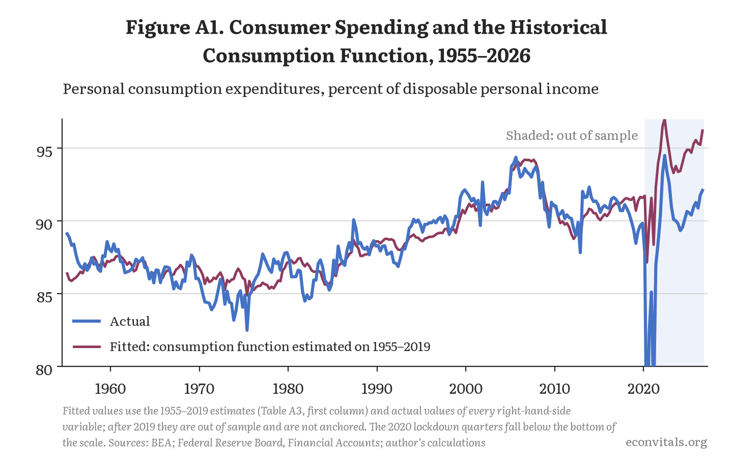
Figure A1 shows the fit. The model tracks the big movements in spending relative to income: the low spending share of the mid-1970s and early 1980s, its rise through 2007 and its drop after the financial crisis. But the residual wanders for years at a time, which is why the Durbin–Watson statistic is only 0.31. In 2013 actual spending was 1.4 points of income above the model; by 2019 it was 2.0 points below, the lowest annual average in the 1955–2019 sample. After 2019, out of sample and without any adjustment, the model runs well above actual spending; its spikes in 2020–2021 come from the income term, as stimulus payments pushed income far above its recent average and back.
Persistent residuals are normal in a levels regression of this kind and do not by themselves make it spurious. The test that matters is whether spending and the wealth ratios share a common trend (are cointegrated), so that the regression describes a stable long-run relationship. The Engle–Granger test passes for 1955–2019 (a statistic of −4.36 against a 5 percent critical value of −4.14), for the full sample and, narrowly, for 1989–2015. It fails for 1990–2019 and 2010–2019, where the variables do not move enough for the test to find the relationship. With cointegration the coefficients are consistent, but with residuals this persistent even Newey–West standard errors probably overstate the precision, so the t-statistics should be read generously. The standard remedy, adding leads and lags of the changes in the wealth ratios (dynamic ordinary least squares), leaves the stock coefficient almost unchanged (2.18 cents; Table A5).
2.3 How fast spending adjusts
The levels regression gives only the long-run effect. Two standard models give the timing (Table A4). In the partial-adjustment model, last quarter’s spending share is added to the levels regression; one minus its coefficient is the share of the remaining gap closed each quarter. Over 1955–2019 that is 27 percent a quarter, so 72 percent of the long-run effect arrives within a year and 92 percent within two. In the error-correction model, the quarterly change in the spending share depends on last quarter’s gap from the levels relationship and on the current change in wealth. It closes only 11 percent of the gap a quarter, but the current change in stock wealth has a large immediate effect, so 58 percent of the long-run effect arrives in the first quarter and 66 percent within a year.
Table A4. How Fast Spending Adjusts to a Permanent Change in Stock Wealth
| Sample | Model | Share of the gap closed each quarter (SE) | Half-life (quarters) | Share of the long-run effect reached (percent) | Long-run effect (cents) | |||
|---|---|---|---|---|---|---|---|---|
| Quarter 1 | Quarter 4 | Quarter 8 | Quarter 12 | |||||
| 1955–2019 | Error correction | 0.112 (0.045) | 5.9 | 58 | 66 | 78 | 85 | 2.22 |
| 1955–2019 | Partial adjustment | 0.271 (0.063) | 2.2 | 27 | 72 | 92 | 98 | 2.45 |
| 1955–2026 | Error correction | 0.094 (0.030) | 7.0 | 78 | 78 | 84 | 89 | 1.15 |
| 1955–2026 | Partial adjustment | 0.215 (0.046) | 2.9 | 22 | 62 | 86 | 95 | 1.92 |
Note: Quarter 1 is the quarter of the change. Error correction: the quarterly change in the spending share on last quarter’s residual from the levels regression, last quarter’s change in the share and the current changes in the wealth ratios and controls; its long-run effect is the levels coefficient, and its large first-quarter share comes from the current change in stock wealth (1.30 cents through 2019). Partial adjustment: the levels regression with last quarter’s spending share added; the speed is one minus that coefficient and the long-run effect is the short-run coefficient divided by the speed. Newey–West standard errors, four lags.
Sources: BEA; Federal Reserve Board, Financial Accounts of the United States; author’s calculations.
Either way, the response is at the fast end of the literature. It is in line with the county estimates of Chodorow-Reich, Nenov and Simsek (complete within about seven quarters) and with the Danish investor data, in which spending starts responding in the first month, and much faster than Fair’s partial-adjustment equations, in which about 45 percent arrives after a year. The post uses the partial-adjustment speed for the consumption function in its Table 1 and Figure 7.
2.4 How much the estimates depend on the specification
Table A5 shows the baseline and 18 variations on it (two of which change only how the standard errors are calculated). Through 2019, the stock coefficient stays between 1.5 and 2.5 cents in every variant but three. Measuring housing as home equity (net of mortgages) raises it to 3.3 cents. Using total net worth instead of the three types gives 2.5 cents per dollar of all wealth. And taking interest and dividends out of income turns it negative (−1.8). That last result is a reason to keep the standard income measure rather than evidence that stock wealth lowers spending: dividends are the cash return on stock wealth, so once they are removed from income the regression credits the spending they finance to the income ratio and cannot separate spending out of dividends from spending out of the stocks that pay them.
Table A5. How the Wealth Coefficients Change With the Specification
| Specification | Stock wealth | Housing wealth | ||
|---|---|---|---|---|
| 1955–2019 | 1955–2026 | 1955–2019 | 1955–2026 | |
| Baseline | 2.22 (0.49) | 1.15 (0.57) | 4.44 (0.72) | 4.20 (0.89) |
| No controls | 1.98 (0.37) | 1.11 (0.46) | 5.40 (0.59) | 4.92 (0.57) |
| Without transfers | 2.32 (0.50) | 1.15 (0.59) | 4.63 (0.59) | 4.21 (0.71) |
| Without unemployment | 2.40 (0.43) | 1.37 (0.51) | 4.54 (0.66) | 4.37 (0.81) |
| Without the real interest rate | 2.07 (0.39) | 1.16 (0.48) | 4.57 (0.79) | 4.19 (0.92) |
| Without income relative to its average | 1.97 (0.43) | 0.97 (0.53) | 5.16 (0.68) | 4.89 (0.79) |
| Adding consumer sentiment | 1.52 (0.45) | 1.16 (0.36) | 4.14 (0.51) | 3.91 (0.55) |
| Adding a level shift from 2009 | 2.09 (0.50) | 0.89 (0.61) | 4.50 (0.77) | 4.33 (0.96) |
| Leads and lags of wealth changes (±2) | 2.18 (0.45) | 1.13 (0.61) | 4.53 (0.68) | 4.28 (0.86) |
| Leads and lags of wealth changes (±4) | 1.95 (0.48) | 1.09 (0.62) | 4.84 (0.77) | 4.84 (0.83) |
| Home equity instead of gross housing | 3.29 (0.55) | 1.13 (0.73) | 5.93 (0.79) | 2.25 (1.98) |
| Total outlays instead of spending | 2.26 (0.50) | 1.08 (0.62) | 5.17 (0.81) | 4.90 (0.97) |
| Income excluding interest and dividends | −1.83 (0.56) | −2.44 (0.52) | 6.35 (0.88) | 6.06 (0.96) |
| Starting in 1965 | 1.58 (0.61) | 0.34 (0.64) | 3.31 (0.53) | 2.89 (0.82) |
| Starting in 1980 | 2.07 (0.50) | 0.80 (0.64) | 2.50 (0.43) | 1.44 (0.97) |
| Standard errors with 4 lags instead of 8 | 2.22 (0.42) | 1.15 (0.48) | 4.44 (0.60) | 4.20 (0.74) |
| Standard errors with 12 lags instead of 8 | 2.22 (0.52) | 1.15 (0.60) | 4.44 (0.79) | 4.20 (0.98) |
| Dropping 2020–2022 entirely | — | 1.18 (0.60) | — | 4.31 (0.89) |
| Total net worth instead of the three types | 2.52 (0.50) | 1.44 (0.56) | — | — |
Note: Cents per dollar; Newey–West standard errors in parentheses. “Leads and lags” is dynamic ordinary least squares. The home-equity row reports home equity (housing minus mortgages) in the housing columns, with mortgages moved out of other wealth. The net-worth row reports the single net-worth coefficient in the stock columns.
Sources: BEA; Federal Reserve Board, Financial Accounts of the United States; author’s calculations.
The pattern that matters most for the post is in the second column. In every specification, adding the years since 2019 cuts the stock coefficient, by about half in most of them and by between a quarter and four-fifths in all, to between 0.3 and 1.4 cents (setting aside the income-excluding-dividends variant). Dropping 2020–2022 entirely instead of using lockdown dummies gives 1.2 cents, so the decline is not an artifact of how the pandemic is handled. Housing is more sensitive to the starting date: starting in 1980 instead of 1955 lowers it from 4.4 to 2.5 cents.
3. How the consumption function has done since 2019
3.1 Method
The out-of-sample exercise in the post’s Figure 5 follows five steps. (1) Estimate the regression on 1955Q1–2019Q4. (2) Compute its fitted spending share for every quarter since, using the actual values of all seven right-hand-side variables. (3) Because the residual wanders (Figure A1), shift the prediction by the average residual of an anchor period so that it matches actual spending then; the main anchor is 2019, whose average residual is −2.01 points of income. The lockdown dummies are not used, so the prediction ignores the lockdowns. (4) Multiply the predicted share by actual disposable income to get predicted spending in dollars. (5) Repeat with stock wealth held at its anchor-period ratio to income to isolate what the model expected stocks to add. Stock wealth rose from 1.81 times disposable income on average in 2019 to 3.06 times in the third quarter of 2026, an excess over the 2019 ratio of $30.2 trillion.
3.2 The projection and why it misses
Anchored to 2019, the model predicts that spending in the third quarter of 2026 would be 94.2 percent of disposable income. Actual spending was 92.1 percent, a shortfall of 2.1 percent of income, or $509 billion at an annual rate (2.3 percent of spending). Table A6 shows the path. The lockdowns dominate 2020 and 2021; the gap nearly closed in 2022, as households spent down the savings they had piled up; it reopened in 2023 and the first half of 2024, and it has been roughly stable since. Summed from the start of 2020, the model overpredicts spending by $3.7 trillion, about 15 percent of a year’s disposable income; summed from the start of 2022, by $1.8 trillion.
Table A6. The 1955–2019 Consumption Function, Year by Year
| Year | Actual spending share | Fitted share | Actual minus fitted | Predicted minus actual, anchored to: | |
|---|---|---|---|---|---|
| 2019 | 2015–2019 | ||||
| 2000 | 91.6 | 91.0 | 0.6 | — | — |
| 2005 | 94.0 | 93.7 | 0.2 | — | — |
| 2007 | 93.4 | 94.1 | −0.8 | — | — |
| 2010 | 90.6 | 90.3 | 0.4 | — | — |
| 2012 | 89.0 | 88.9 | 0.1 | — | — |
| 2013 | 91.9 | 90.5 | 1.4 | — | — |
| 2015 | 90.9 | 90.3 | 0.6 | — | — |
| 2016 | 91.4 | 90.9 | 0.4 | — | — |
| 2017 | 90.9 | 91.3 | −0.3 | — | — |
| 2018 | 90.2 | 91.5 | −1.4 | — | — |
| 2019 | 89.3 | 91.3 | −2.0 | 0.0 | 1.5 |
| 2020 | 82.0 | 90.1 | −8.0 | 6.0 | 7.5 |
| 2021 | 85.8 | 92.4 | −6.5 | 4.5 | 6.0 |
| 2022 | 93.4 | 96.0 | −2.6 | 0.6 | 2.1 |
| 2023 | 90.2 | 93.6 | −3.3 | 1.3 | 2.8 |
| 2024 | 89.9 | 94.2 | −4.3 | 2.3 | 3.8 |
| 2025 | 90.8 | 95.1 | −4.3 | 2.3 | 3.8 |
| 2026 Q3 | 92.1 | 96.2 | −4.1 | 2.1 | 3.6 |
Note: Percent of disposable income (spending share) and percentage points (the rest); annual averages of quarterly values. Fitted values are in sample through 2019. The anchored predictions add the average residual of the anchor period (−2.01 points for 2019, −0.54 for 2015–2019) and ignore the lockdowns, so 2020 and 2021 are dominated by them.
Sources: BEA; Federal Reserve Board, Financial Accounts of the United States; author’s calculations.
Table A7 shows why the model expected spending to rise faster than income. Of the predicted rise in the spending share of 4.9 points ($1,184 billion a year at today’s income), 2.8 points ($672 billion) come from stocks, 1.4 points ($337 billion) from housing and 0.5 points ($122 billion) from income growing more slowly than its recent average. The actual share rose 2.8 points ($675 billion). Comparing actual spending with the version that holds stock wealth at its 2019 ratio, actual spending is $163 billion higher: that is the part of the expected stock effect that is visible, 24 percent of it, or 0.54 cents per dollar of excess stock wealth. That attribution assumes the rest of the model is right. The gap is a residual, and it could equally reflect a smaller housing effect or something the model leaves out.
Table A7. Why the Model Expected Spending to Rise Faster Than Income, 2019 to 2026 Q3
| Variable | 2019 average | 2026 Q3 | Coefficient | Contribution to the spending share (points) | Contribution ($ billions) |
|---|---|---|---|---|---|
| Stock wealth / income | 1.81 | 3.06 | 2.22 | +2.77 | +672 |
| Housing wealth / income | 1.74 | 2.06 | 4.44 | +1.39 | +337 |
| Other net wealth / income | 3.20 | 2.97 | −1.00 | +0.22 | +54 |
| Transfers / income | 19.47 | 21.43 | 0.029 | +0.06 | +14 |
| Unemployment rate | 3.67 | 4.13 | −0.086 | −0.04 | −10 |
| Real 3-month bill rate | 0.63 | 0.31 | 0.065 | −0.02 | −5 |
| Income relative to its 2-year average | 2.95 | 1.24 | −0.293 | +0.50 | +122 |
| Predicted change | +4.89 | +1,184 | |||
| Actual change | 89.3 | 92.1 | +2.79 | +675 | |
| Predicted minus actual | +2.10 | +509 |
Note: Wealth ratios are multiples of income; transfers and the spending share are percent of income. Coefficients on wealth are cents per dollar, on transfers points per point, on the others points per unit. Contribution = coefficient × change; dollars multiply points of income by disposable income in 2026 Q3 ($24.2 trillion, annual rate).
Sources: BEA; Federal Reserve Board, Financial Accounts of the United States; author’s calculations.
3.3 The starting point matters
The choice of anchor matters a great deal (Table A8 and Figure A2). The saving rate was unusually high in 2019, 7.3 percent, and the model’s residual that year was the lowest in the sample, so anchoring to 2019 already builds in a low level of spending. Anchored instead to the 2015–2019 average, when the residual was about −0.5 points, the model is 3.6 percent of income ($865 billion) above actual spending, more than its whole expected stock effect ($699 billion), so actual spending is below even the version of the model that gives stocks no role. Anchoring to individual years from 2015 to 2017 gives shortfalls of 3.8 to 4.7 percent of income.
Table A8. The Projection’s Miss in 2026 Q3 Depends on the Anchor
| Anchor | Saving rate that year (percent) | Anchor (points of income) | Predicted minus actual (percent of income) | Predicted minus actual ($ billions) | What stocks were expected to add ($ billions) | What is visible ($ billions) |
|---|---|---|---|---|---|---|
| 2015 | 5.9 | 0.59 | 4.7 | 1,138 | 746 | −392 |
| 2016 | 5.4 | 0.43 | 4.5 | 1,099 | 759 | −341 |
| 2017 | 5.8 | −0.35 | 3.8 | 911 | 692 | −220 |
| 2018 | 6.4 | −1.35 | 2.8 | 668 | 625 | −43 |
| 2019 | 7.3 | −2.01 | 2.1 | 509 | 672 | 163 |
| 2015–2019 average | — | −0.54 | 3.6 | 865 | 699 | −166 |
| 2022 | 3.5 | −2.60 | 1.5 | 366 | 438 | 72 |
| 2023 | 6.1 | −3.33 | 0.8 | 190 | 575 | 385 |
| 2024 | 6.2 | −4.32 | −0.2 | −52 | 410 | 461 |
Note: The 1955–2019 estimates, shifted by the average residual of the anchor period. “Expected” is the stock coefficient times the rise in stock wealth above its anchor-period ratio to income; “visible” is expected minus the miss, i.e., how far actual spending is above a version of the model with stock wealth held at the anchor ratio. A negative visible effect means actual spending is below even that version. Saving rates are annual averages (BEA).
Sources: BEA; Federal Reserve Board, Financial Accounts of the United States; author’s calculations.
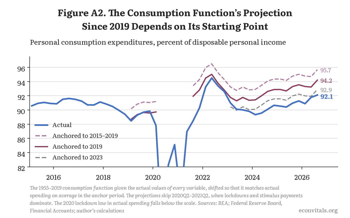
Anchoring to 2023 or 2024 gives a very different answer: a shortfall of 0.8 percent of income, or none at all. Measured from 2023, most of the stock effect the model expects on the gains since then is visible (1.5 cents per dollar); measured from 2024, all of it and more (2.5 cents). Put differently, the shortfall relative to the model is a level that opened up in two stages, between 2013 and 2019 and between 2019 and 2024, and has held steady since, rather than a gap that has kept widening as stocks have risen. Measured over the whole period since before the pandemic, households have spent much less of their stock gains than the 1955–2019 average implies; measured over the last two years alone, their response to the latest gains looks close to normal. That matters for reading the post’s “about 1 cent”: it describes how little of the cumulative run-up since the late 2010s has been spent, which is the relevant comparison if households have been treating that run-up as unreliable, but the response at the margin over 2024–2026 has been closer to 2 cents.
3.4 Other samples, specifications and functional forms
Table A9 repeats the projection for models estimated on other samples and with other specifications, all anchored to 2019. The shortfall ranges from 1.3 to 4.7 percent of income, and the share of the expected stock effect that is visible ranges from none to 57 percent. The model estimated on 1955–2007 shows the smallest shortfall, mainly because spending had already fallen far below that model by 2019 (its anchor is −5.9 points, against −2.0), so anchoring builds in a low level of spending; the home-equity version, which has the largest stock coefficient, shows the largest.
Table A9. The Projection’s Miss Under Other Samples and Specifications (All Anchored to 2019)
| Estimated on | Stock coefficient (cents) | Anchor (points of income) | Predicted minus actual (percent of income) | Predicted minus actual ($ billions) | What stocks were expected to add ($ billions) | Share of that visible (percent) |
|---|---|---|---|---|---|---|
| 1955–2007 | 2.40 | −5.94 | 1.3 | 313 | 725 | 57 |
| 1955–2012 | 2.49 | −5.23 | 1.6 | 388 | 752 | 48 |
| 1955–2016 | 2.30 | −3.33 | 1.9 | 454 | 696 | 35 |
| 1955–2019 (baseline) | 2.22 | −2.01 | 2.1 | 509 | 672 | 24 |
| 1980–2019 | 2.07 | −1.81 | 1.9 | 453 | 626 | 28 |
| 1990–2019 | 2.43 | −1.68 | 3.1 | 740 | 734 | −1 |
| 1955–2019, no controls | 1.98 | −2.08 | 1.5 | 355 | 598 | 41 |
| 1955–2019, leads and lags (±2) | 2.18 | −1.90 | 2.1 | 513 | 661 | 22 |
| 1955–2019, home equity | 3.29 | −2.98 | 4.7 | 1,130 | 996 | −14 |
Note: All in 2026 Q3. A negative share means actual spending is below the version with stock wealth held at its 2019 ratio.
Sources: BEA; Federal Reserve Board, Financial Accounts of the United States; author’s calculations.
The functional form matters too. Models that are linear in dollars, like this consumption function and the simple rules of more than about 2 cents in Section 6.3, overpredict spending since 2019. Models in which spending is proportional to wealth raised to a power do not. A constant-elasticity regression of log spending on log income and log net worth, estimated through 2019, put spending 4.2 percent below its fitted value in 2019 and 4.5 percent below in the latest four quarters: essentially the same relative miss, so the rise in spending since 2019 is about what that model predicts. FRB/US, also constant-elasticity, tracks spending since 2019 closely (Section 6.2). In those models the cents-per-dollar effect falls as wealth rises relative to spending, so they too say that a dollar of stock wealth now carries less spending than it did on average in the past. The two families differ on how much less.
3.5 Is the miss unusual?
To judge whether a 2.3 percent miss after six and three-quarter years is large, the whole procedure was repeated from every anchor year from 1970 to 2019: estimate on 1955 through the anchor year, anchor to that year, feed in the actual data and compare 27 quarters later, the distance from 2019Q4 to 2026Q3 (Figure A3 and Table A10).
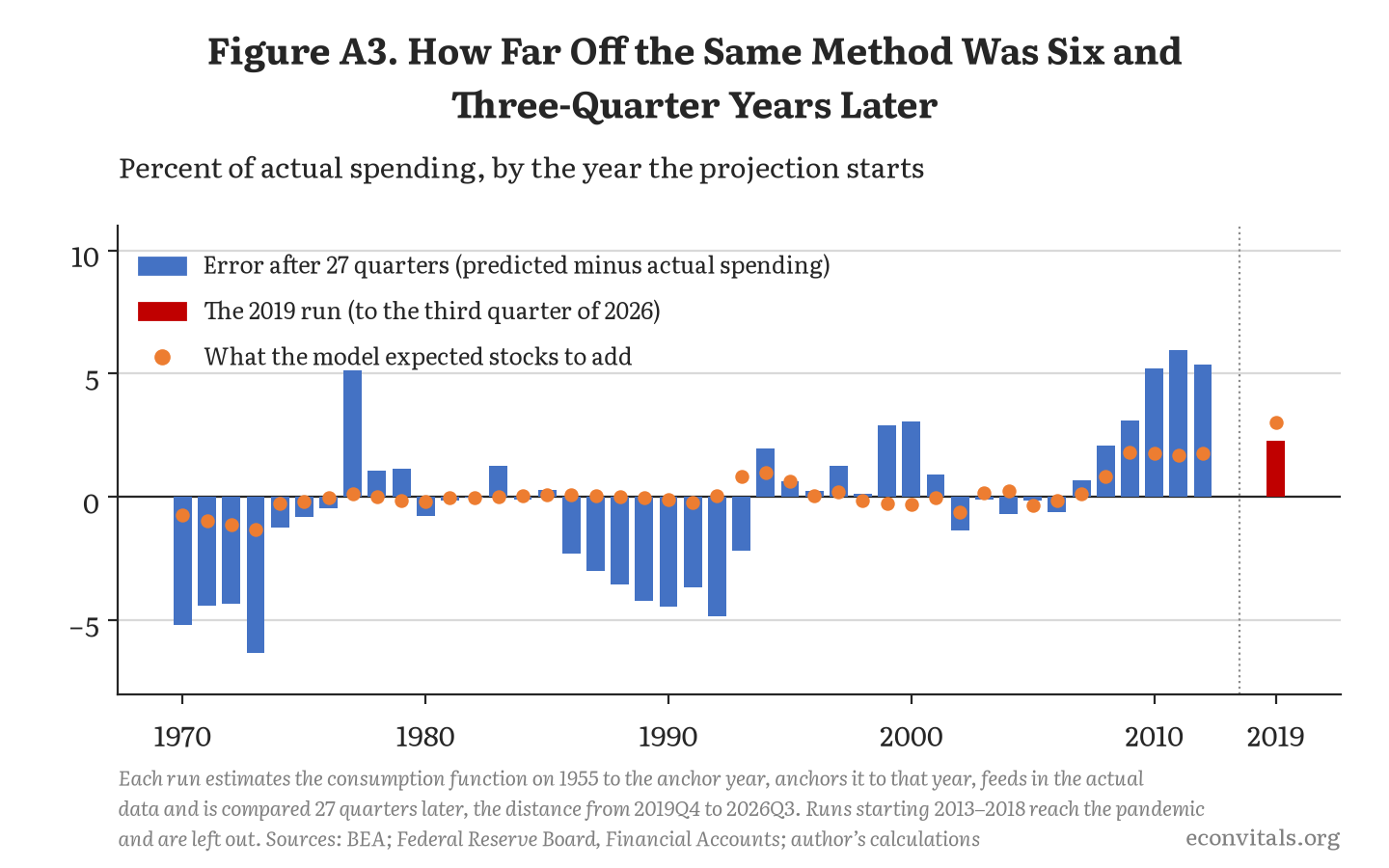
Taken alone, the miss is not unusual for this method. Across the 43 runs from 1970 to 2012, whose windows end before the pandemic, the absolute error after 27 quarters had a median of 1.4 percent, a 75th percentile of 3.9 and a maximum of 6.3; 42 percent of runs missed by at least 2.3 percent in one direction or the other, and 16 percent overpredicted by at least that much. So the gap cannot by itself prove that households held back on spending their gains.
Table A10. How Far Off the Same Method Was Six and Three-Quarter Years Later
| Anchor year | Estimated on | Window | Error at end of window (percent) | What the model expected stocks to add (percent of spending) | Largest error in window (percent) | Average error in window (percent) |
|---|---|---|---|---|---|---|
| 1975 | 1955–1975 | 1976 Q1–1982 Q3 | −0.8 | −0.2 | −4.3 | −2.4 |
| 1980 | 1955–1980 | 1981 Q1–1987 Q3 | −0.8 | −0.2 | 4.5 | 1.2 |
| 1985 | 1955–1985 | 1986 Q1–1992 Q3 | 0.3 | 0.1 | 2.6 | 1.4 |
| 1990 | 1955–1990 | 1991 Q1–1997 Q3 | −4.4 | −0.1 | −4.4 | −2.6 |
| 1995 | 1955–1995 | 1996 Q1–2002 Q3 | 0.6 | 0.6 | 1.8 | 0.1 |
| 1999 | 1955–1999 | 2000 Q1–2006 Q3 | 2.9 | −0.3 | 3.4 | 0.9 |
| 2003 | 1955–2003 | 2004 Q1–2010 Q3 | −0.1 | 0.2 | 3.6 | 1.8 |
| 2007 | 1955–2007 | 2008 Q1–2014 Q3 | 0.7 | 0.1 | −2.8 | −1.3 |
| 2009 | 1955–2009 | 2010 Q1–2016 Q3 | 3.1 | 1.8 | 3.3 | 1.0 |
| 2010 | 1955–2010 | 2011 Q1–2017 Q3 | 5.2 | 1.8 | 5.2 | 2.3 |
| 2011 | 1955–2011 | 2012 Q1–2018 Q3 | 6.0 | 1.7 | 6.0 | 2.8 |
| 2012 | 1955–2012 | 2013 Q1–2019 Q3 | 5.4 | 1.8 | 5.4 | 2.4 |
| 2019 | 1955–2019 | 2020 Q1–2026 Q3 | 2.3 | 3.0 | — | — |
Note: Error = predicted minus actual spending, percent of actual spending, 27 quarters after the anchor year (the distance from 2019 Q4 to 2026 Q3). Across all 43 anchor years from 1970 to 2012 (windows ending before 2020), the absolute error at that point had a median of 1.4 percent, a 75th percentile of 3.9, a 90th percentile of 5.2 and a maximum of 6.3, and the signed error’s correlation with what the model expected stocks to add was 0.70. For the 2019 run the largest errors are in the lockdown quarters, so the window columns are not shown.
Sources: BEA; Federal Reserve Board, Financial Accounts of the United States; author’s calculations.
Two things make that reading more than noise. First, across the pre-2020 runs the error lines up with the model’s own expected stock contribution (correlation 0.7): when the model credits stocks with a lot of extra spending, it tends to overpredict. In the 1990s, when the estimated stock coefficient was near zero, the stock boom produced underpredictions; in the 2010s, with a coefficient of about 2.5 cents, it produced overpredictions of 3 to 6 percent (runs anchored in 2009–2012, compared in 2016–2019). Second, the 2019 run has the largest expected stock contribution of any run (3.0 percent of spending), and its miss is smaller than that contribution, consistent with only part of the stock effect showing up. The same evidence also cuts against treating post-pandemic behavior as new: the model overpredicted the late-2010s stock boom by as much as or more than it overpredicts now. The fairest summary is that for at least a decade households have spent noticeably less out of stock gains than the 1955–2019 average implies.
3.6 What it implies for the wealth effect
Taking the projection at face value, the 2.2 cents the model was estimated with translates into about 0.5 cents of visible spending per dollar of stock gains since 2019, and less than nothing since the 2015–2019 average. That is the basis for the post’s statement that adjusting for the prediction errors takes the 2-cent estimate “down to 1 cent or lower.” The qualifications are the ones above: the attribution to stocks assumes the rest of the model is right, the miss is within the method’s historical error, models with a different functional form fit the period well, and the response since 2023–2024 looks closer to 2 cents. The re-estimates in Section 5, which let the data since 2019 speak directly, point the same way as the projection: about 1 cent on all data since 1955 and less over the last 20 years.
4. Gains versus losses
Two approaches test whether spending responds more to falling stock prices than to rising ones. In the levels version, stock wealth relative to income is split into three parts, each deflated by the PCE price index: accumulated real holding gains since 1952, accumulated real holding losses since 1952 (a negative number) and the remainder (the 1952 stock plus net purchases). In the changes version, the quarterly change in real spending per person is regressed on the current and eight lagged quarterly real holding gains, split by sign, with controls; the sums of the coefficients give the cumulative response after a given number of quarters.
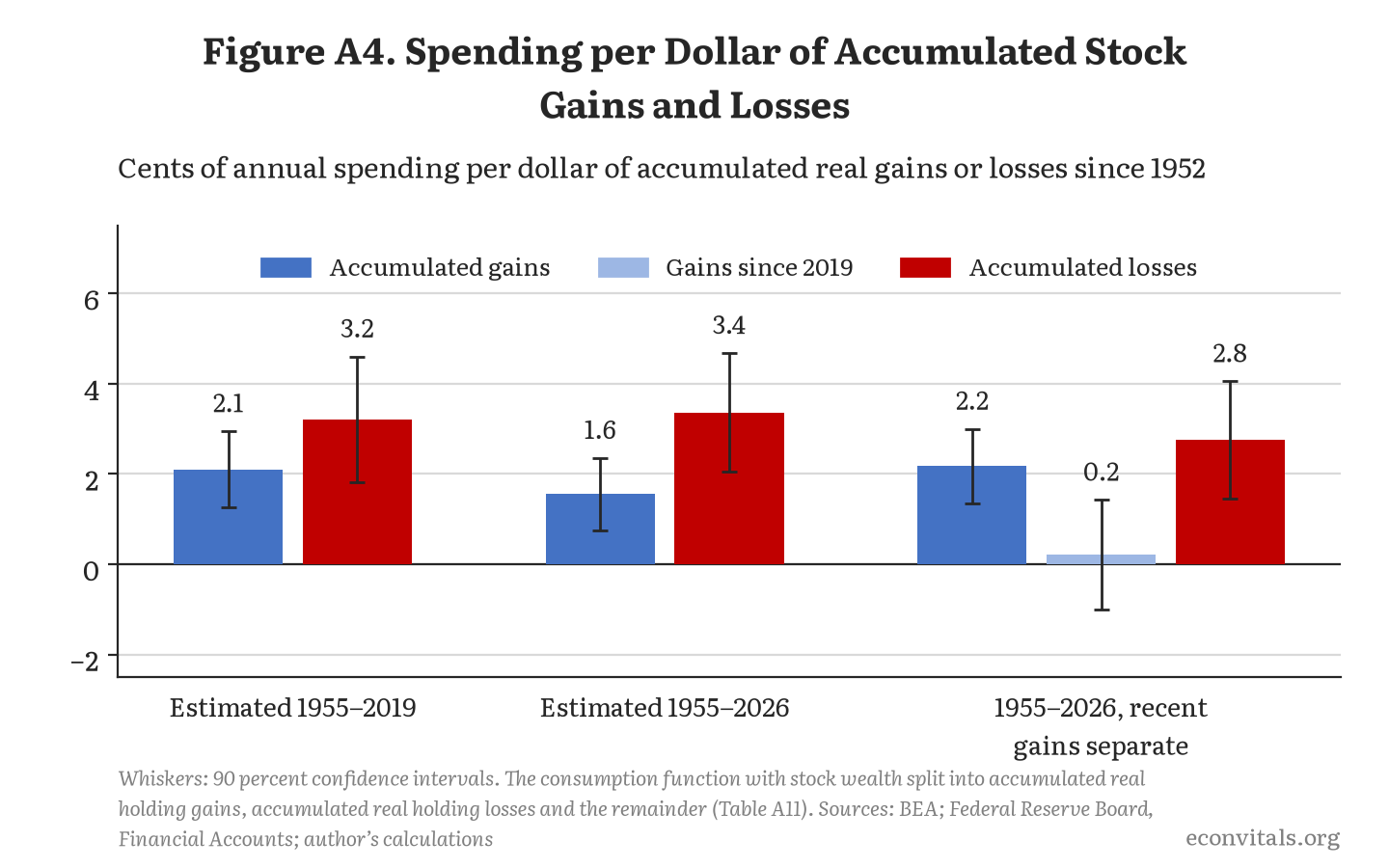
Table A11. Accumulated Stock Gains and Losses Entered Separately
| Sample | Accumulated gains (cents) | Accumulated losses (cents) | t-statistic, gains minus losses | Gains since 2019 (cents) | Housing (cents) |
|---|---|---|---|---|---|
| 1955–2019 | 2.10 (0.51) | 3.21 (0.85) | −1.34 | — | 4.70 (0.76) |
| 1955–2026 | 1.55 (0.49) | 3.36 (0.80) | −3.03 | — | 4.31 (0.79) |
| 1955–2026, gains since 2019 separate | 2.17 (0.50) | 2.76 (0.79) | −0.74 | 0.21 (0.74) | 4.46 (0.79) |
Note: The consumption function with stock wealth relative to income split into accumulated real holding gains since 1952, accumulated real holding losses since 1952 (a negative number) and the remainder (the 1952 stock plus net purchases). In the last row, gains are split into those through 2019 and those from 2020 on. Newey–West standard errors in parentheses.
Sources: BEA; Federal Reserve Board, Financial Accounts of the United States; author’s calculations.
In levels through 2019, a dollar of accumulated losses moves spending somewhat more than a dollar of accumulated gains (3.2 against 2.1 cents), but the difference is well within the margin of error (t = −1.3). Through 2026 the gap widens and becomes significant (3.4 against 1.6 cents, t = −3.0), but only because the unspent gains since 2019 pull the gains coefficient down. Give the post-2019 gains their own coefficient and they get 0.2 cents, earlier gains 2.2 and losses 2.8, and the difference between earlier gains and losses is no longer significant (t = −0.7). The variants in Table A12 tell the same story. Through 2019, stock moves over the past two years matter more than older ones, in both directions and by similar amounts (1.9 cents extra for losses, 2.3 for gains), and the extra effect of accumulated losses, or of being below the previous peak, is not significant. The loss terms stand out only once the post-2019 data are included.
Table A12. Extra Effects of Losses and Gains on Top of Stock Wealth
| Variant | Sample | Stock wealth (cents) | Extra terms (cents) |
|---|---|---|---|
| Cumulative losses since 1952 (extra effect) | 1955–2019 | 2.11 | losses 1.10 (t = 1.6) |
| Cumulative losses since 1952 (extra effect) | 1955–2026 | 1.31 | losses 2.07 (t = 3.2) |
| Losses and gains over the past 2 years (extra effects) | 1955–2019 | 1.50 | losses 1.93 (t = 2.1); gains 2.29 (t = 2.2) |
| Losses and gains over the past 2 years (extra effects) | 1955–2026 | 1.13 | losses 2.74 (t = 3.7); gains 0.38 (t = 0.3) |
| Losses and gains over the past 3 years (extra effects) | 1955–2019 | 1.52 | losses 1.38 (t = 1.8); gains 1.68 (t = 1.9) |
| Losses and gains over the past 3 years (extra effects) | 1955–2026 | 1.03 | losses 2.53 (t = 3.8); gains 0.81 (t = 0.8) |
| Shortfall from the previous peak (extra effect) | 1955–2019 | 1.73 | losses 1.25 (t = 1.4) |
| Shortfall from the previous peak (extra effect) | 1955–2026 | 0.28 | losses 2.63 (t = 2.9) |
Note: Each extra term enters alongside total stock wealth, so it measures the effect beyond the average. Losses are negative numbers, so a positive coefficient means losses lower spending by more than the average. The shortfall from the previous peak is real stock wealth per person below its previous high, scaled by income.
Sources: BEA; Federal Reserve Board, Financial Accounts of the United States; author’s calculations.
Table A13. The Changes Model: Cumulative Response of Spending to Real Gains and Losses
| Sample | Quarters after | Gains (cents) | Losses (cents) | t-statistic, gains minus losses |
|---|---|---|---|---|
| 1955–2019 | 0 | 1.32 (0.61) | 0.85 (0.73) | 0.41 |
| 1955–2019 | 1 | 2.05 (0.85) | 1.84 (1.09) | 0.13 |
| 1955–2019 | 2 | 2.24 (0.93) | 3.26 (1.50) | −0.49 |
| 1955–2019 | 4 | 2.30 (1.24) | 2.66 (1.72) | −0.14 |
| 1955–2019 | 8 | 3.60 (1.40) | −1.00 (1.62) | 2.18 |
| 1955–2026 | 0 | 1.45 (0.51) | 0.10 (0.64) | 1.45 |
| 1955–2026 | 1 | 2.03 (0.76) | 0.68 (0.90) | 1.00 |
| 1955–2026 | 2 | 2.05 (0.88) | 1.60 (1.18) | 0.27 |
| 1955–2026 | 4 | 2.15 (1.14) | 1.24 (1.52) | 0.39 |
| 1955–2026 | 8 | 3.47 (1.07) | −1.38 (1.36) | 2.90 |
Note: The quarterly change in real spending per person regressed on the current and eight lagged quarterly real holding gains on stocks, housing and other wealth (stocks split by sign), with income growth and changes in unemployment and the real interest rate. Cents of spending per dollar of gain or loss, summed over the current and following quarters. Newey–West standard errors (four lags) in parentheses.
Sources: BEA; Federal Reserve Board, Financial Accounts of the United States; author’s calculations.
The changes model (Table A13) points the other way, if anything. Through 2019 the first-year responses are similar: 2.3 cents for gains and 2.7 for losses after four quarters. With the full sample, gains run ahead (2.1 against 1.2). In both samples the effect of losses fades to nothing by two years while that of gains keeps building, and only that eight-quarter difference is significant. The county estimates in Section 5.3 also find a larger point estimate for gains than for losses (2.9 against 0.2 cents), not significant. None of this supports the idea that households cut back more when stocks fall than they spend when stocks rise, which is why the post uses the same propensity in both directions.
5. Has the effect changed over time?
5.1 Rolling and expanding samples
The same regression was estimated on every 10-, 15- and 20-year window and on every sample starting in 1955 (an expanding window). Table A14 shows selected results and Figure A5 the expanding window, which is the cleanest picture. In samples ending anywhere from 2000 to 2019, the stock coefficient stays between 2.2 and 2.9 cents (2.8 through 1999, 2.5 through 2012, 2.2 through 2019). It then slides as the post-2019 quarters come in: 2.0 through 2023, 1.7 through 2024, 1.3 through 2025 and 1.1 through the third quarter of 2026. Dropping 2020 and 2021 entirely gives 1.2. Housing barely moves, from 4.4 through 2019 to 4.2.
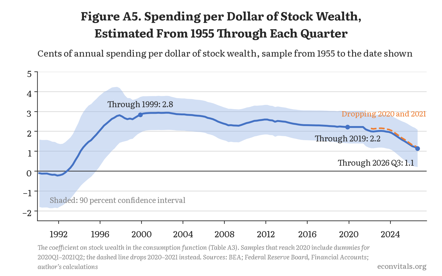
Table A14. The Stock Coefficient Estimated on Different Samples
| Sample ends | Stock wealth (cents) | Housing (cents) | |||
|---|---|---|---|---|---|
| From 1955 | Last 20 years | Last 15 years | Last 10 years | From 1955 | |
| 1999 Q4 | 2.84 (0.55) | 2.23 (0.77) | 0.65 (1.07) | 0.75 (0.35) | 5.87 (1.49) |
| 2007 Q4 | 2.40 (0.51) | 0.42 (0.38) | 0.73 (0.42) | 1.32 (0.35) | 4.69 (0.77) |
| 2012 Q4 | 2.49 (0.45) | 2.00 (0.25) | 2.12 (0.28) | 2.18 (0.52) | 4.57 (0.70) |
| 2015 Q4 | 2.32 (0.46) | 2.07 (0.26) | 1.71 (0.56) | 3.11 (0.53) | 4.54 (0.70) |
| 2019 Q4 | 2.22 (0.49) | 2.70 (0.47) | 2.70 (0.80) | 1.50 (0.46) | 4.44 (0.72) |
| 2021 Q4 | 2.05 (0.52) | 0.58 (1.17) | 0.40 (1.43) | −1.46 (0.95) | 4.30 (0.72) |
| 2023 Q4 | 1.97 (0.51) | 0.11 (1.08) | −0.83 (0.85) | −1.94 (1.02) | 4.10 (0.75) |
| 2024 Q4 | 1.67 (0.55) | −0.06 (0.71) | −1.00 (0.58) | −0.57 (0.33) | 4.00 (0.82) |
| 2025 Q4 | 1.34 (0.59) | 0.27 (0.61) | −0.36 (0.53) | −0.38 (0.31) | 4.12 (0.87) |
| 2026 Q3 | 1.15 (0.57) | 0.62 (0.57) | 0.49 (0.64) | 0.36 (0.58) | 4.20 (0.89) |
Note: The consumption function (Table A3) on samples ending at the date shown. Newey–West standard errors in parentheses. Samples that reach 2020 include the lockdown dummies. Dropping 2020–2021 entirely instead, the estimate through 2026 Q3 is 1.19 from 1955 and 1.19 over the last 20 years.
Sources: BEA; Federal Reserve Board, Financial Accounts of the United States; author’s calculations.
Ten-year windows are unusable: before 1999 the stock coefficient ranges from −5.3 to 12.0 cents, and even windows ending 2010–2019 run from 1.3 to 3.4. With 20-year windows, the estimates settle down in the 2000s and 2010s: 2.0 to 2.7 cents for windows ending 2012–2019. Once a window includes more than a year or so of data since 2019, the estimate falls to roughly zero: −0.1 to 0.9 cents for 20-year windows ending from the third quarter of 2021 on (0.6 for the latest, 2006Q4–2026Q3, or 1.2 without 2020–2021), and −1.6 to 0.5 for 15-year windows. The post’s Figure 6 shows the 20-year version.
The changes model tells a similar story by era. With four lags of stock and housing gains and recent income growth, the response to stock gains after four quarters is 5.1 cents (standard error 1.2) over 1955–1989, 3.1 (0.8) over 1990–2008, 3.4 (1.0) over 2009–2019 and 1.7 (1.1) over 2021Q3–2026Q3: lower in the latest period, but not by enough to be distinguished from the earlier ones on five years of data.
5.2 Break tests
Formal tests for a single break at an unknown date (Table A15) allow every coefficient to change and compare the largest Wald statistic over all candidate dates with critical values from Andrews (1993). On the full sample the test finds a significant break in the stock coefficient, dated 2013Q4 (2.5 cents before, essentially zero after) or, with more of the sample trimmed from each end, 2008Q2. But the search cannot place a break later than 2019Q2 (or 2012Q1), so the “after” period always includes the post-2019 data. Confined to data through 2019, the test picks its very first candidate, 1964Q4, a move from a negative coefficient to a positive one that reflects the early years rather than a decline.
Table A15. Tests for One Unknown Break in a Wealth Coefficient
| Coefficient | Sample | Dates searched | Most likely break | Sup-Wald statistic | Critical values (10 / 5 / 1 percent) | Before (cents) | After (cents) |
|---|---|---|---|---|---|---|---|
| Stocks | full sample | 1962 Q1–2019 Q2 | 2013 Q4 | 13.1 | 7.58 / 9.11 / 12.59 | 2.50 | 0.09 |
| Housing | full sample | 1962 Q1–2019 Q2 | 2019 Q1 | 14.7 | 7.58 / 9.11 / 12.59 | 4.44 | 0.83 |
| Stocks | full sample, 20% trimming | 1969 Q2–2012 Q1 | 2008 Q2 | 10.2 | 6.73 / 8.28 / 11.71 | 2.36 | 0.00 |
| Housing | full sample, 20% trimming | 1969 Q2–2012 Q1 | 2009 Q1 | 12.2 | 6.73 / 8.28 / 11.71 | 4.66 | −1.44 |
| Stocks | through 2019 | 1964 Q4–2010 Q1 | 1964 Q4 | 12.0 | 7.12 / 8.68 / 12.16 | −2.20 | 1.61 |
| Housing | through 2019 | 1964 Q4–2010 Q1 | 1987 Q4 | 10.8 | 7.12 / 8.68 / 12.16 | 6.29 | 2.07 |
Note: Every coefficient may change at the break; the statistic is the largest Wald statistic for a change in the named coefficient over all candidate dates, compared with Andrews (1993, corrected 2003) critical values. The share of the sample trimmed from each end sets how close to the ends a break may fall; the critical values assume stationary regressors, so they are approximate here.
Sources: BEA; Federal Reserve Board, Financial Accounts of the United States; author’s calculations.
Table A16. Breaks at Given Dates, With and Without the Years Since 2019
| Break at | Before (cents) | After, data through 2019 | Wald | After, data through 2026 Q3 | Wald |
|---|---|---|---|---|---|
| 2008 Q2 | 2.36 | 0.68 (47 quarters) | 6.2 | 0.00 (74 quarters) | 10.2 |
| 2010 Q1 | 2.37 | 1.50 (40 quarters) | 1.8 | 0.22 (67 quarters) | 7.3 |
| 2013 Q4 | 2.50 | 1.43 (25 quarters) | 1.2 | 0.09 (52 quarters) | 13.1 |
Note: All coefficients may change at the break date. For a date chosen in advance (2010 Q1 here) the 5 percent critical value is 3.84; for a date found by searching (2008 Q2 and 2013 Q4 were picked by the tests in Table A15), compare with the Andrews values of 7 to 9 there.
Sources: BEA; Federal Reserve Board, Financial Accounts of the United States; author’s calculations.
Table A16 separates the two by fixing the break dates. Using only data through 2019, the stock coefficient after 2010 or after 2013 is about 1.5 cents, and the change is far from significant (Wald statistics of 1.8 and 1.2). After 2008 it is 0.68 cents, a Wald statistic of 6.2: significant for a date picked in advance, not for one found by searching. Add the years since 2019 and all three become large: the 2008 and 2013 breaks, which a search would find, pass the Andrews test, and the 2010 break passes the test for a date chosen in advance. So there is no statistically robust evidence that the stock coefficient fell before 2020. The point estimates for the post-2008 years are lower than the long-run average, though, and the out-of-sample record in Section 3.5 points the same way, so a decline in the 2010s cannot be ruled out. The decline the data can actually detect arrives with the post-2019 observations.
5.3 A check from county data
Rebuilding the county design with public data
The county design of Chodorow-Reich, Nenov and Simsek can be rebuilt from public data: IRS county dividend income (from which stock wealth is estimated by capitalizing dividends, adjusted for each county’s age mix and for stock held in retirement accounts), county payrolls from the Bureau of Labor Statistics and the Survey of Consumer Finances, with Robert Shiller’s and Kenneth French’s returns standing in for the proprietary CRSP data. The rebuild matches the paper on total payroll (1.9 against 2.2 basis points) and employment, but comes in lower on payroll in retail, restaurants and hotels, the number that reads as the propensity to spend: 1.9 against 3.2. So the county-implied effect is about 2 cents per dollar, or 2 to 3 allowing for the gap.
The rebuild extends the paper’s data, which use dividends through 2015, to stock moves through mid-2024. It finds no weakening before 2020: the response is 0.6 cents for stock moves in 1992–2004 and 2.5 cents for moves in 2005–2018, larger in the second half in every variant but one, as in the paper’s own split. The design cannot say much about the 2020s. The pandemic hit restaurant and retail jobs hardest in the dense, rich counties where stock wealth is concentrated, just as the market crashed and recovered, so every stock move whose window touches 2020–2022 has to be dropped, leaving only five clean quarters (2023Q2–2024Q2). Estimated in one regression with the pre-COVID years, those quarters give 1.6 cents, the same as before, but with a 95 percent confidence interval from about −1.5 to 4.6; estimated on their own with 2015–2018, the point estimate is negative (−2.6) and even less precise.
Table A17. The County Design: Local Payrolls Seven Quarters After a Stock Market Move
| Sample | Payroll in retail, restaurants and hotels (≈ cents per dollar) | Total payroll |
|---|---|---|
| Chodorow-Reich, Nenov and Simsek (2021), as published | 3.24 (1.01) | 2.18 (0.63) |
| Rebuild, same years | 1.9 (0.9) | 1.9 (0.9) |
| Rebuild, 1992–2018 moves | 1.7 (0.8) | 1.8 (0.8) |
| First half, 1992–2004 | 0.6 (0.9) | 0.5 (1.0) |
| Second half, 2005–2018 | 2.5 (1.3) | 2.6 (1.3) |
| Rebuild, all years through mid-2024, 2020–2022 out | 1.6 (0.8) | 1.8 (0.7) |
| Rebuild, the five clean quarters since COVID (2023Q2–2024Q2), pooled with 1992–2018 | 1.6 (1.6) | 1.1 (1.2) |
| Rebuild, 1992–2018: market up | 2.9 (1.3) | 2.3 (1.3) |
| Rebuild, 1992–2018: market down (27 of 105 quarters) | 0.2 (1.2) | 1.3 (1.1) |
Note: Basis points of payroll per stock-market gain equal to 1 percent of a county’s annual labor income, which in the paper’s calibration reads as cents of household spending per dollar of stock wealth. Standard errors, clustered by county and quarter, in parentheses. Each row is its own regression, except the post-COVID row, which is estimated together with the pre-COVID years (only the stock coefficient differs between the two periods), and the market-up and market-down rows, which split the stock move by the sign of the quarter’s return in one regression.
Sources: Chodorow-Reich, Nenov and Simsek (2021); IRS Statistics of Income county data; BLS Quarterly Census of Employment and Wages; Survey of Consumer Finances; author’s calculations.
6. The post’s other three approaches
6.1 The back-of-the-envelope calculation
The simplest calculation in the post divides the rise in spending as a share of disposable income by the rise in household stock wealth as a multiple of income. From 2015–2019 to the first three quarters of 2026, spending rose from 90.5 to 91.6 percent of income, about 1 point, while stock wealth rose from 1.76 to 2.81 times income, about one year’s income. One extra point of spending per extra year of income in stock wealth is 1 cent per dollar. Table A18 shows how the answer depends on the base period.
Table A18. The Back-of-the-Envelope Calculation From Different Starting Points
| Base period | Spending share in base (percent of income) | Stock wealth in base (multiple of income) | Cents of spending per dollar of extra stock wealth | ||
|---|---|---|---|---|---|
| To 2026 so far | To 2026 Q3 | To 2026 so far, net of housing | |||
| 2000–2019 | 91.3 | 1.45 | 0.2 | 0.5 | −0.5 |
| 2010–2019 | 90.6 | 1.55 | 0.8 | 1.0 | −0.6 |
| 2015–2019 | 90.5 | 1.76 | 1.0 | 1.2 | −0.3 |
| 2015 | 90.9 | 1.67 | 0.6 | 0.9 | −0.9 |
| 2016 | 91.4 | 1.64 | 0.2 | 0.5 | −1.1 |
| 2017 | 90.9 | 1.77 | 0.6 | 0.9 | −0.6 |
| 2018 | 90.2 | 1.89 | 1.5 | 1.7 | 0.3 |
| 2019 | 89.3 | 1.81 | 2.3 | 2.2 | 1.0 |
| 2022 | 93.4 | 2.24 | −3.3 | −1.6 | −1.8 |
| 2023 | 90.2 | 1.99 | 1.7 | 1.8 | 1.9 |
| 2024 | 89.9 | 2.29 | 3.3 | 2.9 | 3.8 |
Note: The rise in spending as a share of disposable income from the base period to 2026, divided by the rise in household stock wealth as a multiple of income. In the first three quarters of 2026 the spending share averaged 91.6 percent and stock wealth 2.81 times income; in the third quarter alone, 92.1 and 3.06. “Net of housing” first takes off the rise in housing wealth times the consumption function’s housing coefficient (4.4 cents). Stock wealth is measured at the start of each quarter.
Sources: BEA; Federal Reserve Board, Financial Accounts of the United States; author’s calculations.
Single years can mislead because the saving rate moves around for reasons that have nothing to do with stocks. Measured to the third quarter of 2026, the calculation gives 0.9 cents from a 2015 base, 2.2 from 2019, less than nothing from 2022 and 2.9 from 2024. The 2019 saving rate was unusually high (7.3 percent), which makes 2019 a low base for spending and the answer high; in 2022 households were spending down their pandemic savings (the saving rate was 3.5 percent), which makes the answer negative. The post therefore uses the five years before the pandemic. Longer pre-pandemic bases give similar or smaller answers: 0.8 cents from 2010–2019 and 0.2 cents from 2000–2019. Recent bases give larger ones, 1.7 cents from 2023 and 3.3 from 2024 (to 2026 so far), for the reason discussed in Section 3.3: the response to the latest gains looks closer to normal even though the level of spending relative to wealth is low. The last column credits housing with the consumption function’s 4.4 cents per dollar before attributing the rest to stocks. Since home values also rose, that leaves stocks with nothing or less from the multi-year pre-pandemic bases (and 1 cent from 2019), which is why the post says “and probably less.”
6.2 The Federal Reserve’s model since 2019
FRB/US is the Federal Reserve Board’s large-scale model of the U.S. economy, and the post’s Figure 5 compares its prediction for spending since 2019 with what happened. The model’s spending equations set a target for consumption that depends on households’ expected (“permanent”) labor, transfer and property income and on their net worth, with an elasticity of 0.187 on net worth. Spending on nondurables and services closes about 16 percent of the gap to that target each quarter, with momentum from its own recent growth, and about 30 percent of it follows current income one for one. The exercise runs the model’s consumption equations by hand on the Board’s published data (the data package of November 4, 2026, with history through 2026Q2), from 2019Q4 onward with the actual paths of income, wealth and the model’s other inputs. Spending on durable goods and on other goods and services is simulated with each equation’s residual set to its 2015–2019 average (the durables residual has been persistently negative, so zero residuals would bias it); housing services are taken as given, and total spending is aggregated with the model’s own weights.
The model tracks spending closely. In the second quarter of 2026 its prediction was within $33 billion, 0.15 percent, of actual spending, and since the third quarter of 2022 it has never been off by more than 0.64 percent. Summed from the start of 2020 it overpredicts spending by $1.5 trillion, almost all of it during the pandemic; summed from the start of 2022, by $0.17 trillion. Households never made up the spending they missed during the lockdowns, which is why the post says FRB/US may if anything overstate the wealth effect.
The post’s statement that FRB/US has a marginal propensity to consume of 0.9 cents in the short run and 1.4 in the long run comes from the Econvitals Macroeconomic Simulator’s runs of the full model. After a permanent 25 percent fall in stock prices, which takes $18.5 trillion from households, real consumer spending is 0.78 percent lower after a year and 1.18 percent lower after five years in the version in which investors expect lower earnings: $175 billion and $263 billion at today’s spending, or 0.9 and 1.4 cents per dollar lost. In the version in which investors demand a higher return, which also raises businesses’ cost of capital, the figures are 1.0 and 1.6 cents. These responses include everything else in the model, notably the Federal Reserve cutting interest rates in response, which is one reason they are smaller than the roughly 2.1 cents per dollar that the 0.187 elasticity implies at today’s ratio of spending to net worth before any feedback.
6.3 Simple rules
Table A19 compares actual spending since 2019 with the consumption function, FRB/US and three simple rules. Each rule starts from the 2019 spending share of income and adds a fixed number of cents per dollar of stock wealth above its 2019 ratio to income, all at once. A 1-cent rule underpredicts spending in the third quarter of 2026 by $373 billion, a 3-cent rule overpredicts it by $232 billion and a 5-cent rule by $837 billion. A rule of 2.2 cents fits exactly from a 2019 start; quarter by quarter, the rule that fits has been between 1.7 and 2.9 cents since late 2024, mostly close to 2, and a single rule fitted to every quarter since 2023 is 2.1 cents. As Table A18 shows, the same arithmetic from a 2015 start gives 0.9 cents.
Table A19. Consumer Spending Since 2019 Compared With What Six Models Predict
| Model | Spending growth since 2019 (percent) | Predicted minus actual ($ billions, annual rate) | Predicted minus actual (percent of income) | Cumulative since 2022 Q1 ($ billions) |
|---|---|---|---|---|
| Actual | 54.5 | — | — | — |
| Consumption function (estimated 1955–2019) | 58.1 | +509 | +2.1 | +1,783 |
| Spend 1 cent per dollar of stock gains | 52.0 | −373 | −1.5 | −1,281 |
| Spend 3 cents per dollar | 56.2 | +232 | +1.0 | −145 |
| Spend 5 cents per dollar | 60.3 | +837 | +3.5 | +991 |
| No wealth effect (2019 spending share) | 49.9 | −675 | −2.8 | −1,848 |
| Fed’s model (FRB/US), through 2026 Q2* | 52.6* | +33* | — | +174* |
Note: 2019 to 2026 Q3, current dollars. Disposable income rose 50 percent and household stock wealth went from 1.81 to 3.06 times income. Each model starts from actual spending in 2019 and is given what actually happened to income and wealth. The rules add the stated cents per dollar of stock wealth above its 2019 ratio to income, immediately, to spending that otherwise keeps its 2019 share of income; a rule of 2.2 cents matches spending exactly. *FRB/US ends in the second quarter of 2026, the last quarter in the Fed’s data (actual growth to then: 52.3 percent).
Sources: BEA; Federal Reserve Board, Financial Accounts and FRB/US; author’s calculations.
7. From spending to GDP: how the post’s Table 1 is built
The post’s Table 1 translates each approach into the hit to GDP growth over the year after a fall in stock prices. Households held $74.0 trillion of stock at the end of the second quarter of 2026, so a 25 percent fall takes $18.5 trillion, a 35 percent fall $25.9 trillion and a 50 percent fall $37.0 trillion; GDP is $33.0 trillion at an annual rate. Table A20 gives the arithmetic, to two decimals, and for the 25 percent case the path over five years.
Table A20. The Arithmetic Behind the Post’s Table 1
| Fall in the stock market | FRB/US | Spend 1 cent per dollar | Consumption function (2.2 cents, phased in) | Spend 3 cents per dollar | |
|---|---|---|---|---|---|
| Lower earnings | Higher required return | ||||
| 25 percent ($18.5 trillion) | 0.43 | 0.57 | 0.56 | 0.89 | 1.68 |
| 35 percent ($25.9 trillion) | 0.60 | 0.80 | 0.78 | 1.25 | 2.35 |
| 50 percent ($37.0 trillion) | 0.86 | 1.15 | 1.12 | 1.78 | 3.36 |
| 25 percent fall, by horizon | |||||
| After 1 year | 0.43 | 0.57 | 0.56 | 0.89 | 1.68 |
| After 2 years | 0.55 | 0.84 | 0.56 | 1.14 | 1.68 |
| After 3 years | 0.58 | 1.00 | 0.56 | 1.22 | 1.68 |
| After 5 years | 0.53 | 1.15 | 0.56 | 1.24 | 1.68 |
Note: Reduction in the level of real GDP relative to a world without the fall, percent; the post reads the one-year number as the cut in growth over the next year. Household stock wealth is $74.0 trillion (Financial Accounts, 2026 Q2) and GDP $33.0 trillion (2026 Q3, annual rate). The rules divide the cut in annual spending by GDP; the consumption function phases 2.22 cents in at its estimated partial-adjustment speed (27 percent of the remaining gap each quarter, 72 percent within a year). FRB/US is the Econvitals Macroeconomic Simulator’s permanent 30 percent fall, scaled to 25 percent and to today’s stock wealth, with the Fed responding and imports absorbing part of the spending cut; the 35 and 50 percent rows scale it proportionally.
Sources: Federal Reserve Board, Financial Accounts and FRB/US; BEA; author’s calculations.
The two rule columns take the whole cut in annual spending in the first year: 1 cent per dollar of $18.5 trillion is $185 billion, 0.56 percent of GDP, and 3 cents is 1.68 percent. The consumption-function column applies the 1955–2019 estimate of 2.2 cents, phased in at its partial-adjustment speed: 72 percent of the long-run effect within a year, or 0.89 percent of GDP, rising to 1.24 percent in the long run. None of the three has a response from the Federal Reserve or an allowance for the share of spending that goes to imports, so they overstate the hit to GDP relative to a full model. The FRB/US columns come from the Simulator, which includes both: 0.43 percent of GDP after a year in the version in which investors expect lower earnings and 0.57 percent in the version in which they demand a higher return, rising to 0.58 and 1.0 percent after three years. The post treats the reduction in the level of GDP after a year as the reduction in growth over that year, and scales the FRB/US results proportionally for the 35 and 50 percent falls. The post’s preferred case, 1 cent per dollar, gives 0.6 percentage point for a 25 percent fall; its severe case, 3 cents with a 50 percent fall, gives 3.4.
8. Data and replication
Every input is public. The regressions use the Federal Reserve’s Financial Accounts of the United States (release of September 11, 2026, through the second quarter of 2026: Tables B.101, B.101.e and R.101, now distributed as S1M_b, S1M_e_b and S1M_r), the Bureau of Economic Analysis’s national income and product accounts through the third quarter of 2026 (Tables 2.1, 2.3.4, 2.3.5 and 2.3.6) and, from FRED, the unemployment rate and the three-month Treasury bill rate. FRB/US comes from the Board’s public model package, and the stock-fall scenarios from the Econvitals Macroeconomic Simulator. The ownership shares cited in the post come from the Board’s Distributional Financial Accounts; the 2001 forecast from the December 2000 Greenbook and the first-published national accounts from the Philadelphia Fed’s Real-Time Data Set for Macroeconomists; the stock market declines from Kenneth French’s data library; and the fortunes of the ten richest Americans from Forbes. The county rebuild uses the IRS’s county income data, the BLS Quarterly Census of Employment and Wages and the Survey of Consumer Finances.
The replication package contains the frozen data, the code that builds the quarterly panel from these sources, the scripts that produce every table and figure in the post and in this appendix, and a check that compares their output with the numbers printed here.
References
- Aladangady, Aditya, and Laura Feiveson. 2018. “A Not-So-Great Recovery in Consumption: What Is Holding Back Household Spending?” FEDS Notes, Federal Reserve Board. Link.
- Aladangady, Aditya. 2017. “Housing Wealth and Consumption: Evidence from Geographically Linked Microdata.” American Economic Review 107 (11). Working paper.
- Andersen, Asger Lau, Niels Johannesen and Adam Sheridan. 2024. “Dynamic Spending Responses to Wealth Shocks: Evidence from Quasi Lotteries on the Stock Market.” American Economic Review: Insights 6 (3). Link.
- Andersen, Henrik Yde, and Søren Leth-Petersen. 2021. “Housing Wealth or Collateral: How Home Value Shocks Drive Home Equity Extraction and Spending.” Journal of the European Economic Association 19 (1). Link.
- Andrews, Donald W. K. 1993. “Tests for Parameter Instability and Structural Change with Unknown Change Point.” Econometrica 61 (4); corrected 2003, Econometrica 71 (1). Link.
- Apergis, Nicholas, and Stephen M. Miller. 2006. “Consumption Asymmetry and the Stock Market: Empirical Evidence.” Economics Letters 93 (3). Working paper.
- Baker, Malcolm, Stefan Nagel and Jeffrey Wurgler. 2007. “The Effect of Dividends on Consumption.” Brookings Papers on Economic Activity 2007 (1). Link.
- Beach, Samara, William Gamber and Patrick Moran. 2025. “Wealth Heterogeneity and Consumer Spending.” FEDS Notes, Federal Reserve Board. Link.
- Bigot, Sixtine, and Aurélien Espic. 2026. “Are Stock Market Valuations Fuelling US Consumption?” Banque de France Eco Notepad 454. Link.
- Buiter, Willem H. 2008. “Housing Wealth Isn’t Wealth.” NBER Working Paper 14204. Link.
- Calomiris, Charles W., Stanley D. Longhofer and William Miles. 2013. “The Housing Wealth Effect: The Crucial Roles of Demographics, Wealth Distribution and Wealth Shares.” Critical Finance Review 2 (1). Link.
- Carroll, Christopher D., Misuzu Otsuka and Jiri Slacalek. 2011. “How Large Are Housing and Financial Wealth Effects? A New Approach.” Journal of Money, Credit and Banking 43 (1). Link.
- Case, Karl E., John M. Quigley and Robert J. Shiller. 2005. “Comparing Wealth Effects: The Stock Market versus the Housing Market.” Advances in Macroeconomics 5 (1). Link.
- Case, Karl E., John M. Quigley and Robert J. Shiller. 2013. “Wealth Effects Revisited: 1975–2012.” Critical Finance Review 2 (1). Link.
- Chodorow-Reich, Gabriel, Plamen T. Nenov and Alp Simsek. 2021. “Stock Market Wealth and the Real Economy: A Local Labor Market Approach.” American Economic Review 111 (5). Link.
- Davis, Morris A., and Michael G. Palumbo. 2001. “A Primer on the Economics and Time Series Econometrics of Wealth Effects.” Finance and Economics Discussion Series 2001-09, Federal Reserve Board. Link.
- Di Maggio, Marco, Amir Kermani and Kaveh Majlesi. 2020. “Stock Market Returns and Consumption.” Journal of Finance 75 (6). Working paper.
- Donihue, Michael R., and Andriy Avramenko. 2007. “Decomposing Consumer Wealth Effects: Evidence on the Role of Real Estate Assets Following the Wealth Cycle of 1990–2002.” B.E. Journal of Macroeconomics 7 (1). Working paper.
- Duca, John V., John Muellbauer and Anthony Murphy. 2017. “Wealth Effects (Plural) and U.S. Consumer Spending.” Paper presented at the 2018 American Economic Association meetings. Link.
- Fagereng, Andreas, Martin Blomhoff Holm, Benjamin Moll and Gisle Natvik. 2019. “Saving Behavior Across the Wealth Distribution: The Importance of Capital Gains.” NBER Working Paper 26588 (revised 2025). Link.
- Fair, Ray C. 2017. “Household Wealth and Macroeconomic Activity: 2008–2013.” Journal of Money, Credit and Banking 49 (2–3). Link.
- Fair, Ray C. 2024. Macroeconomic Modeling: The Cowles Commission Approach. MIT Press. Draft.
- Guren, Adam M., Alisdair McKay, Emi Nakamura and Jón Steinsson. 2021. “Housing Wealth Effects: The Long View.” Review of Economic Studies 88 (2). Working paper.
- JPMorganChase Institute (Chris Wheat, George Eckerd and Melissa O’Brien). 2026. “More U.S. Households Are Supporting Spending by Drawing on Investment Wealth.” Link.
- Lettau, Martin, and Sydney C. Ludvigson. 2004. “Understanding Trend and Cycle in Asset Values: Reevaluating the Wealth Effect on Consumption.” American Economic Review 94 (1). Working paper.
- Ludvigson, Sydney, and Charles Steindel. 1999. “How Important Is the Stock Market Effect on Consumption?” Federal Reserve Bank of New York Economic Policy Review 5 (2). Link.
- Ludwig, Alexander, and Torsten Sløk. 2002. “The Impact of Changes in Stock Prices and House Prices on Consumption in OECD Countries.” IMF Working Paper 02/1. Link.
- Mehra, Yash P. 2001. “The Wealth Effect in Empirical Life-Cycle Aggregate Consumption Equations.” Federal Reserve Bank of Richmond Economic Quarterly 87 (2). Link.
- Mian, Atif, and Amir Sufi. 2011. “House Prices, Home Equity–Based Borrowing, and the US Household Leverage Crisis.” American Economic Review 101 (5). Link.
- Mian, Atif, Kamalesh Rao and Amir Sufi. 2013. “Household Balance Sheets, Consumption, and the Economic Slump.” Quarterly Journal of Economics 128 (4). Link.
- Mitra, Indrajit, and David Rapach. 2026. “Downside Risk to the Stock Market and Consumption.” Federal Reserve Bank of Atlanta Policy Hub. Link.
- Poterba, James M. 2000. “Stock Market Wealth and Consumption.” Journal of Economic Perspectives 14 (2). Link.
- Sinai, Todd, and Nicholas S. Souleles. 2005. “Owner-Occupied Housing as a Hedge Against Rent Risk.” Quarterly Journal of Economics 120 (2). Working paper.
- Slacalek, Jiri. 2009. “What Drives Personal Consumption? The Role of Housing and Financial Wealth.” B.E. Journal of Macroeconomics 9 (1). Working paper.
- van Treeck, Till. 2008. “Asymmetric Income and Wealth Effects in a Non-Linear Error Correction Model of U.S. Consumer Spending.” IMK Working Paper 6/2008. Link.